Read on Ordinary Analysis

I related a lot to the essay by Anurag Verma. He argued that most of our readings are utility driven i.e. we read because we have to.

Among all these debates and discussions, I felt we were missing one point: how is India different from other nations?

I don’t have a lot of foreign associates. But from the little knowledge, it didn’t feel like others were drowning themselves in books while India alone wasn’t reading. It is a contemporary issue that transcends borders, regions and seas.

So the question arose:

How do Indians read compared to other countries?

And the only way we can answer this is through data.

I looked at this from two angles:

• What is the buying pattern of different countries with respect to genre?
• How much, on average, is an Indian spending on trade books?

Let’s dissect the first one:

In terms of revenue share, Indians are spending far more on educational books than the US, UK or European countries. So Anurag’s point is not completely wrong. And intuitively, that makes sense.

But now, let’s look at it from another angle: as a percentage of GDP, how much are Indians spending on trade books (i.e. excluding educational books)?

An average Indian is actually spending more on trade books than an average US and European citizen. But less than the UK.

This shows that when it comes to buying non-educational books, Indians are more intentional compared to more developed nations. When you are spending more of your hard-earned money, especially in a country with a lower per-capita GDP, you need to be more intentional.

One methodological note: this analysis uses nominal GDP per capita as the denominator. Book prices vary across markets. A $10 US paperback might be ₹400-600 in India, depending on the publisher and format - but books are globally traded goods with some price convergence, unlike purely local services. Using nominal figures keeps the comparison straightforward, though a full PPP adjustment could be explored in future work.

As usual, reality is far from a clean black-and-white thing. It is much more nuanced. On average, Indians tend to read more for utility, but we also tend to spend more on non-utility books.

This also raises an interesting question: what happens when India’s per capita GDP rises? More surplus should lead to more spending on pleasure?

Notes & Sources

Trade books are commercially published books sold to the general public, excluding educational textbooks, academic journals, and professional reference materials. In this analysis, trade books = Fiction + Non-Fiction.

Data note: All book market figures reflect 2024 actuals from industry sources (Horizon Databook, FEP, Nielsen). GDP per capita figures are from 2024-2025; US figures use 2025 IMF projections. Year-on-year differences are negligible (<2%) and do not materially affect the conclusions.

Calculation methodology: Trade book spending per capita was derived by multiplying total market size by the trade book revenue share (Fiction + Non-Fiction %), then dividing by population. This was then expressed as a percentage of nominal GDP per capita.

The plot uses the mean of each range as the representative value.

India

• Market size: $10.37B (Horizon Databook) [1]
• Educational: 60.2% mean revenue share (Horizon [1], IBEF [2])
• Fiction: 17.5% revenue share, +30.7% YoY growth [1][2]
• Children’s: 9.8% revenue share [1]

United States

• Market size: $40.44B (Horizon Databook) [3]
• Fiction: 32.8% ($3.26B), +12.6% YoY (AAP) [4]
• Children’s: 24.7% [3]
• Educational: 19.8% [3]
• Non-Fiction: 19.2% ($2.88B), +1.3% YoY (AAP) [4]
• Religious/Professional: 3.5% [3]

United Kingdom

• Market size: £1.82B physical (Nielsen) [5]
• Fiction: 42.5% mean revenue share, record high, +18% YoY [6]
• Non-Fiction: 27.5% [7]
• Educational: 17.4% (Horizon) [8]
• Children’s: 12.6% [5][8]

Europe

• Market size: €24.9B (FEP) [9]
• Fiction: 27.5% [9]
• Educational: 23.3% mean (FEP [9], Horizon [10])
• Non-Fiction: 22.5% [9]
• Academic/Professional: 16.7% [9]
• Children’s: 14.6% [9]

Citations

[1] Grand View Research/Horizon Databook. India Books Market Size & Outlook, 2025–2033. https://www.grandviewresearch.com/horizon/outlook/books-market/india

[2] IBEF. India’s Meteoric Rise as a Publishing Hub. https://www.ibef.org/blogs/india-s-meteoric-rise-as-a-publishing-hub

[3] Grand View Research/Horizon Databook. US Books Market Size & Outlook, 2025–2033. https://www.grandviewresearch.com/horizon/outlook/books-market/united-states

[4] AAP via Publishing Perspectives. December StatShot: US Book Market Up 6.5% Year-to-Date. https://publishingperspectives.com/2025/03/aaps-december-statshot-us-market-up-6-5-percent-year-to-date/

[5] Nielsen BookData. Bestsellers & trends in the UK & Ireland in 2024. https://nielseniq.com/global/en/insights/commentary/2025/bestsellers-trends-in-the-uk-ireland-in-2024/

[6] Friedman, Jane. Book sales update: UK market. https://janefriedman.com/book-sales-update-uk-market/

[7] LoveReading. Fiction Book Sales in 2024 Top The Lot. https://www.lovereading.co.uk/blog/fiction-book-sales-in-2024-top-the-lot-while-non-fiction-lags-behind-9226

[8] Grand View Research/Horizon Databook. UK Books Market Size & Outlook, 2025–2033. https://www.grandviewresearch.com/horizon/outlook/books-market/uk

[9] Federation of European Publishers (FEP). European Book Publishing Statistics 2024. https://www.fep-fee.eu/European-Book-Publishing-Statistics-2024

[10] Grand View Research/Horizon Databook. Europe Books Market Size & Outlook, 2025–2033. https://www.grandviewresearch.com/horizon/outlook/books-market/europe

As an Analytics professional, it is our job not to accept whatever is propagated by the belief system blindly. Rather, do our investigation, and then accept, reject, or refine it.

So, I thought, what if we try to see what is actually happening here? In this blogpost, I will discuss my approaches for the same.

But before asking any questions - let’s have a look at the data. What is the gap between the Conte of domestic league and Europe?

For our analysis, we have also taken Pep and Klopp (Liverpool & Dortmund) - so that we can understand how he compares with the other two. This will help us in putting things into more context.

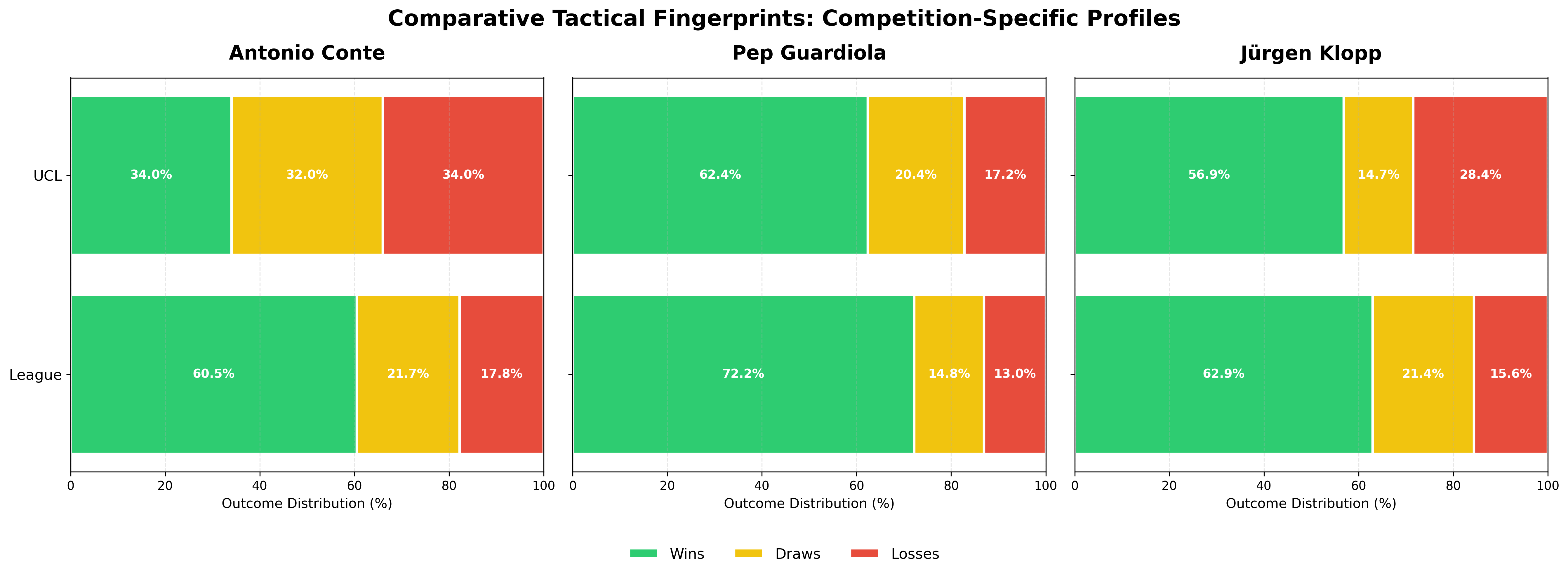
As we can see, there is a significant difference in the win % for Conte - compared to Klopp & Pep.

So the question arises:

Is this a fluke or statistically significant?

A simple Z-test can tell us if the gap in Europe vs Domestic League is just a fluke or if there is some statistical significance.

Turns out - it is highly significant!

The difference is even significant for Pep. Now if you think about it - that is expected. UCL is a tougher competition. So, we would expect to see some reduction in the winning percentage.

For Klopp, though, it is not significant.

┌───────────┬───────────────┬──────────────────┬─────────────┬──────────┬──────────────────────────────┐
│  Manager  │ UCL Win Rate  │ League Win Rate  │ Z-statistic │ P-value  │       Interpretation         │
├───────────┼───────────────┼──────────────────┼─────────────┼──────────┼──────────────────────────────┤
│   Conte   │     34.0%     │      60.5%       │    3.661    │ 0.000251 │ Highly significant difference│
├───────────┼───────────────┼──────────────────┼─────────────┼──────────┼──────────────────────────────┤
│ Guardiola │     62.4%     │      72.2%       │    2.540    │ 0.011086 │   Significant difference     │
├───────────┼───────────────┼──────────────────┼─────────────┼──────────┼──────────────────────────────┤
│   Klopp   │     56.9%     │      62.9%       │    1.161    │ 0.245760 │  No significant difference   │
└───────────┴───────────────┴──────────────────┴─────────────┴──────────┴──────────────────────────────┘

How different are the tactical profiles?

In the first section, we looked at winning % only. Now, let’s examine the complete tactical profile - how the full distribution of wins, draws, and losses shifts between competitions.

The Chi-square test helps us understand if the entire result pattern changes, not just the win rate. And interestingly, even Klopp shows a significant difference here despite his Z-test being non-significant. This suggests his teams play differently in Europe (fewer draws, more decisive results), even though his overall win rate stays similar.

┌───────────┬───────────┬──────────┬────────────┬──────────────────────────────┐
│  Manager  │    χ²     │ P-value  │ Cramér's V │       Interpretation         │
├───────────┼───────────┼──────────┼────────────┼──────────────────────────────┤
│   Conte   │   14.136  │ 0.000852 │   0.145    │ Highly significant difference│
├───────────┼───────────┼──────────┼────────────┼──────────────────────────────┤
│ Guardiola │    6.441  │ 0.039928 │   0.092    │   Significant difference     │
├───────────┼───────────┼──────────┼────────────┼──────────────────────────────┤
│   Klopp   │   10.336  │ 0.005696 │   0.127    │   Significant difference     │
└───────────┴───────────┴──────────┴────────────┴──────────────────────────────┘

So far, all three managers show some form of difference between their league and UCL performances. But here’s the key question: Is the difference abnormal, or is it just the “Elite Tax” of playing in Europe?

The Elite Tax: Accounting for Expected Difficulty

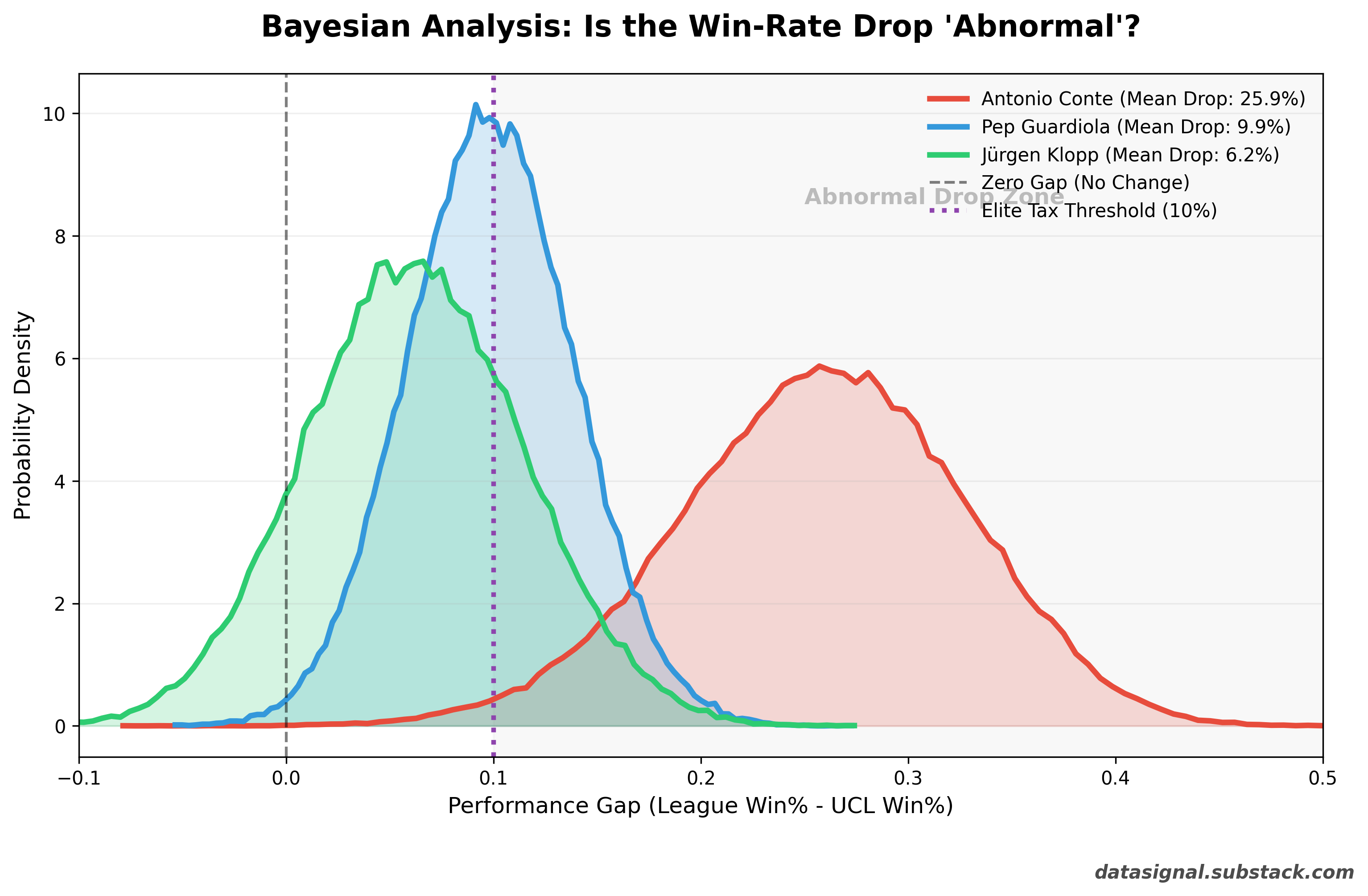
Now, let’s switch from a frequentist lens to a Bayesian one.

Here’s the fundamental insight: UCL is harder than domestic leagues. You can’t really treat playing Everton and Real Madrid at the same level. So we should expect some performance drop when managers face Europe’s elite. The question isn’t “is there a difference?” but rather “is the difference larger than expected?”

The Methodology: The 10% ROPE

I introduced a Region of Practical Equivalence (ROPE), which I call the “Elite Tax.” I am granting every manager a “pardon” for a 10% drop in win rate. If their win rate drops by 10% or less, we consider that a normal byproduct of elite competition.

I then ran 100,000 simulations for each manager to calculate the probability that their performance drop is abnormal (greater than 10%).

If a manager’s drop is within the 10% zone → Normal (performing as expected given increased difficulty)
If a manager’s drop exceeds 10% → Abnormal (genuine UCL problem)

The Results

┌───────────┬───────────┬────────────────────┬──────────────────────────────────┐
│  Manager  │ Mean Drop │ P(Exceeds 10% Tax) │         Interpretation           │
├───────────┼───────────┼────────────────────┼──────────────────────────────────┤
│   Conte   │   25.9%   │      98.76%        │ Abnormal UCL underperformance    │
├───────────┼───────────┼────────────────────┼──────────────────────────────────┤
│ Guardiola │    9.9%   │      48.36%        │ Normal (within expected range)   │
├───────────┼───────────┼────────────────────┼──────────────────────────────────┤
│   Klopp   │    6.1%   │      23.18%        │ Normal (well within range)       │
└───────────┴───────────┴────────────────────┴──────────────────────────────────┘

What This Means

Pep Guardiola: The Benchmark. Pep’s distribution is centered almost perfectly on our 10% “Elite Tax” line. With a 48% chance of exceeding that threshold, his performance is essentially a coin flip. Mathematically, he is performing exactly how an elite manager should in a tougher competition.

Jürgen Klopp: The Outlier (The Good Kind). Klopp’s entire distribution is tucked safely to the left of the 10% line. There is only a 23% chance that his drop-off is abnormal. But here’s the interesting part: his Z-test showed no significant win rate difference, yet his Chi-square test was significant. Why? Because his tactical approach shifts in Europe - fewer draws, more decisive results - even though his overall win rate stays similar. He doesn’t win less in the Champions League; he just plays differently. More high-stake matches, all-or-nothing football. If anything, Klopp is competition-proof; his tactical identity survives the jump from domestic leagues to Europe better than Pep or Conte.

Antonio Conte: The “Statistical Glitch.” Conte lives in a different zip code. With 98.7% certainty, the model confirms that his European drop-off is abnormal. Even after accounting for his smaller UCL sample size (which makes his curve wider), there is almost zero overlap between his reality and that of Pep or Klopp.

How to read the plot: Don’t just look at the peaks of the curves. Look at where they don’t overlap. Pep and Klopp’s performance distributions live in the same neighborhood. Conte’s distribution doesn’t even have a view of their street.

The Verdict

Statistics confirm what the eye test suggested: Only Conte has a genuine UCL problem.

While all three managers show some performance difference between competitions (as they should - the UCL is harder), only Conte’s gap is abnormal after accounting for the increased difficulty. Pep and Klopp are performing within the expected range for elite managers facing elite opposition.

The “Tale of Two Contes” is a real, quantifiable pattern that has persisted across 50 Champions League matches and 618 league games. Whether it’s tactical inflexibility in knockout rounds, squad depth issues, or something else entirely - the numbers make one thing clear: domestic dominance doesn’t automatically translate to European success.

Link to the notebook: https://github.com/shibaprasadb/datasignal/blob/main/conte_record/conte_record.ipynb

This needed production-level accuracy. But the simple API approach wasn’t cutting it. After testing 50 cases, I was only hitting around ~75% accuracy (37 out of 50). For production, that’s a non-starter.

The Problem with Single API Calls

The LLM was doing the task correctly for some instances but missing elements in others. Sometimes it would catch all 10 items, other times only 7 or 8. The pattern was clear: when it failed, it undercounted. It never hallucinated extra elements or went above the true count. It just missed things.

This directional bias turned out to be the key insight.

So I “Random Forest” It

I decided to apply the “wisdom of crowds” principle. The same concept that makes Random Forest work. Instead of relying on a single API call, use multiple calls and aggregate intelligently.

The evaluation rule was simple: Max(API_call_1, API_call_2, …, API_call_n)

Example: If there are 10 elements and three API calls return [7, 10, 3], the final output is 10.

Why this works: The undercounting errors get filtered out. The max function naturally finds the correct answer as long as at least one call succeeds. Since the LLM never overcounts, the highest value is almost always the right one.

Here’s how the two approaches compare:

The Math Behind It

With a single API call, the question is: What’s the probability of success?

With ensemble, it becomes: What’s the probability of at least one success?

The math changes drastically:

P(at least one correct) = 1 - P(all calls wrong)

For n=3 calls with p=0.75 success rate:

• P(all wrong) = (1-p)ⁿ = 0.25³ = 0.015625
• P(at least one correct) = 1 - 0.015625 = 98.4%

Going from 75% to 98.4% with just 3 calls? Not bad at all.

Finding the Sweet Spot

But I couldn’t just pick any number. Each API call costs money and adds latency. I needed to balance accuracy against cost.

Here’s how the numbers break down:

The diminishing returns kick in hard after n=3. Going from 98.4% to 99.6% costs an entire extra API call for just 1.2 percentage points. But for production-level reliability, I decided that extra margin was worth it.

I settled on n=4: 99.6% accuracy at 4x the cost.

When This Breaks

This approach only works because my LLM had a directional bias (like undercounting - in this case). The evaluation function must match your error pattern:

• Undercounting errors → Use Max()
• Overcounting errors → Use Min()
• Random errors (sometimes high, sometimes low) → Use majority voting with odd n (3, 5, 7) to avoid ties

The key is understanding how your model fails, not just that it fails. Directional biases can take many forms - summarization models that are consistently too brief, classifiers that favor certain categories, extractors that miss edge cases. Each needs its own aggregation strategy.

If you don’t understand your failure mode, you’re just burning money on redundant calls.

(Now that I think about it, we can dedicate a separate blog post on designing Eval functions)

The Takeaway

Sometimes the best solution isn’t a better prompt or a bigger model. It’s understanding your failure mode and exploiting it mathematically.

A single API call gave me 75% accuracy. Four calls with a simple Max() aggregator got me to 99.6%. Same model, same prompt. Just a smarter approach.

The real lesson? When you can’t improve the model’s performance, improve how you use it. In a constrained space, solving a problem becomes more interesting.

Still, the 3 lakh number is huge. Especially when we are far from hitting below the replacement level TFR. In any case, I got curious and wanted to explore what is happening with other states.

State Selection

Taking a look at 28 states would increase the noise more than the signal. And I don’t intend to publish a comprehensive comparative study of all the states. So, I cherry-picked a few, just to see how they’re doing:

• Tamil Nadu: Often cited as a model state for educational outcomes. Good to have them as a benchmark.
• Bihar: Eastern Indian state, West Bengal’s neighbor. Most populous state in the East. The lowest per capita income in the country.
• Maharashtra: Western Indian state. Highest state GDP. Mix of urban and rural demographics.
• Haryana: Northern Indian state. 7th richest in terms of per capita income.
• Uttar Pradesh: Bihar’s neighbor. 2nd most populous state overall. Similar socio-economic profile to Bihar in many ways.

This selection gives us a mix of geographical regions, economic profiles, and educational performance levels - enough to see if West Bengal’s trend is an outlier or part of a broader pattern.

Let’s have a look at the absolute numbers - and their trends.

(Note: the numbers are quite decentralized. So I had to collate them from several sources. Directionally, this should be quite accurate.)

Absolute Numbers: Trends from 2021–2025

What stands out:

For Haryana and West Bengal, there has been a decline for 2 consecutive years. But others have shown a consistent pattern overall. For UP, the pattern is interesting - there’s some volatility, but it is still stable. No sharp decline like West Bengal.

The West Bengal drop is particularly dramatic: from approximately 800K students in 2021 to around 470K in 2025. That’s a 41% decline. Haryana shows a similar downward trend, though less severe - from about 230K to 195K (a 15% drop).

Maharashtra, Tamil Nadu, Bihar, and Uttar Pradesh remain relatively stable, with only minor fluctuations around their baseline numbers.

Summary: Year-on-Year Changes

The table makes it clear: West Bengal’s decline is not just steep, it’s an outlier. No other state comes close to this magnitude of drop.

Normalizing by Population

Let’s take a look at the number of exam takers per 1,000 population:

Data Signals:

Maharashtra maintains the highest rate throughout (around 12–13 students per 1,000 population), suggesting either better retention rates or favorable demographics. West Bengal’s rate drops dramatically from about 8 to under 5 per 1,000 population - confirming that this isn’t just a population effect, but a real decline in participation rates.

This chart reveals interesting patterns, but comes with a caveat. This has an implicit assumption: the proportion of the eligible age group (16-18 year-olds) within the total population is uniform across states. Which, obviously, is not true. States with younger populations will have proportionally more children under 10 and fewer teenagers, while states further along in demographic transition will have a higher share of the 16-18 cohort. But we don’t have more granular data readily available. At least, I couldn’t find one. Ideally, we should be looking at the base of 16-20 or 15-19 age cohorts. That would give us a better idea about the “eligible” group.

Another Proxy: Youth Population Base

The closest we can get to the ideal metric is the population of the 0–14 age group in 2021, which was published by Data for India. This can serve as a reasonable proxy for the eligible age group in 2025.

What if we try to see the number of students appearing per 1,000 youth?

What this reveals:

It looks far worse for West Bengal. But this is a total guesstimation - at best. Here, ‘Youth’ is proxied by the 0–14 population share in 2021. By 2025, this group spans roughly ages 4–18. It’s not a perfect match to the Class 12 eligible cohort (≈17–18 years), but directionally it reflects the size of the feeder base.

Maharashtra leads with 58.0 students per 1,000 youth, followed by Tamil Nadu (50.0) and Uttar Pradesh (37.7). West Bengal sits at just 22.6 - trailing behind Haryana (26.7).

This stark difference (58.0 for Maharashtra vs 22.6 for West Bengal) suggests one of two things:

• Massive dropout rates between lower and upper secondary levels in West Bengal
• Demographic differences - West Bengal might have a younger age structure with proportionally more children in the 0–10 range than the 10–14 range

Most likely, it’s a combination of both.

What Could Be Happening?

The 2017 Policy and the Overage Bulge

If the age mandate was introduced in 2017, requiring students to be 10 years old in Class 5, those students would hit Class 12 around 2024–2025. The timing checks out perfectly.

But here’s a critical question: Was there a bulge of overage students in earlier years that’s now correcting?

In many Indian states, particularly in rural areas, it’s not uncommon for children to start school late or repeat grades. If West Bengal had a significant population of unqualified students in the system pre-2017, the 2021–2023 cohorts might have represented this bulge working its way through. The 2024–2025 drop could then be the system “normalizing” to age-appropriate enrollments.

This would explain why the drop is so dramatic - it’s not just one year’s worth of students, but potentially 2–3 years’ worth of overage students who would have been in the system under the old regime.

Why Haryana?

Haryana’s decline is notable but less discussed. I haven’t found evidence of a similar age-mandate policy there. This warrants investigation. Possible factors could include:

• Migration patterns (families moving for work)
• Shift to private schooling or alternative examination boards (CBSE, ICSE)
• Economic factors affecting school retention

Future Work

This exploratory analysis raises more questions than it answers (which has been my goal anyways for this newsletter):

• Granular age-cohort data: Getting actual 15–19 or 16–20 population data by state would dramatically improve the accuracy of per-capita calculations.
• Covid’s shadow: Does the pandemic have something to do with this? The 2024-2025 cohort would have been in Classes 9-10 during 2020-2021 (peak Covid years). If the pandemic disproportionately affected rural schooling (due to a lack of digital infrastructure), we might see this reflected in the numbers. Breaking down the data by urban-rural divide would help determine if Covid-induced dropouts are part of the story.
• Pre-2017 enrollment patterns: Analyzing the age distribution of students in West Bengal’s secondary schools from 2015–2020 would reveal if there was indeed an overage bulge.
• Dropout analysis: Where exactly are students dropping out? Between Class 8–10? Or 10–12? State-level progression ratios would be illuminating.
• Cross-board comparison: Many students in urban areas take CBSE/ICSE boards instead of state boards. Are West Bengal’s numbers declining while CBSE enrollment is rising?
• Haryana deep-dive: Understanding what’s driving Haryana’s decline could reveal factors beyond policy changes - economic trends, migration patterns, or shifts in educational preferences.
• Long-term tracking: Will West Bengal’s numbers stabilize at this new lower level, or continue to decline? Data from 2026–2027 will be crucial.

Conclusion

West Bengal’s ~37% decline in Class 12 exam takers from 2024 to 2025 is unprecedented among major Indian states. While the 2017 age-mandate policy provides a plausible explanation - a correction after years of unqualified students in the system - the sheer magnitude demands deeper investigation.

As someone from West Bengal, these numbers are both surprising and worrying. They point to deeper structural issues in educational access, retention, or migration that go beyond a single policy change. Whether this is a one-time correction or the beginning of a longer-term trend will become clearer in the years ahead.

If you found this worth your time, please subscribe to The Data Signal - it’s free. I explore data, AI, analytics, and strategy, tackling interesting questions that don’t have obvious answers. It would mean the world to me, knowing that someone is finding value in my work.

On the days I am at the office, I prefer to have lunch in the office cafeteria. It is generally either chicken kebabs and roti or a chicken salad - both good, high-protein options.

Last week, I saw something interesting. There was a biryani counter on an unusual day (we generally have biryani on Wednesdays). The sign said, “Calcutta style Biryani — biryani with potatoes (alu)”.

I got excited and went for it, instead of my usual lunch. It was a complete disaster. They had just added potatoes to some form of biryani. The biryani was spicier than a typical Andhra-style biryani, and the overall taste was quite bad. I regretted taking in approximately 700 calories for nothing.

Later, while thinking about the biryani, I suddenly remembered Catenaccio, the football formation made famous by Helenio Herrera when he was at Inter. The legendary Inter team, playing that formation, went on to play three European finals back-to-back and won two.

There have been enough write-ups about the famous formation and style of play, but to give a brief summary: it became famous as a defensive formation. But it had another element to it: the quick attack. Herrera apparently gave strong instructions to his players that when they got the ball, they had to move it as quickly as possible into the opponents’ half with as few touches as possible.

After Herrera, many tried to replicate the system but failed miserably. Herrera himself once explained why people failed to replicate it:

The problem is that most of the people who copied me copied me wrongly. They forgot to include the attacking principles that my Catenaccio included.

This is essentially what happened with the “Calcutta Biryani” at my office cafeteria. They were busy replicating the USP (adding potatoes) but miserably failed to replicate the other things that make Calcutta biryani what it is: soft, fluffy rice, light spices, and diverse ingredients.

This is something that I feel is more common than we realize, especially in the business world and in daily life. Organizations try to mimic others’ success by only replicating their USP. And they miss out on the nuances that made the business what it is.

For example, the McPizza from McDonald’s, the Zune from Microsoft, among many other cases.

When copying success, we gravitate toward the obvious differentiator: the potatoes, the defensive setup, the standout feature. But we ignore the invisible supporting structures that actually make it work. Copy the whole system, not just the part everyone notices. Call it the Catenaccio Principle.

This piece was first written for my ‘Ordinary Analysis’ newsletter. Read it there.

I am fairly comfortable using them as a co-pilot: I design everything, solve smaller tasks with them, and then patch everything together.

Over the weekend, I did some vibe-coding, coupled with my old style of using LLMs, to create my professional website. I had tried doing something like this long back, but my lack of knowledge in HTML/CSS was holding me back. So I had a very basic WordPress page. Thanks to LLMs, I could easily create my website.

Here are some notes and observations:

Importance of software engineering

I am not a software engineer in any shape or form. I just have a basic understanding because of my work, and that proved to be quite crucial in this whole exercise. The biggest hurdle I found while doing vibe-coding was that the code wasn’t modular enough most of the time. I had to give constant nudges like this:

And once prompted, it did a good job of modifying.

Smaller chunks, small tasks

Be it vibe-coding or simple prompting, I never try to do multiple things in one go. I break down the bigger task into smaller buckets, then ask the LLM to perform those smaller tasks. In that way, things don’t break. It is also quite easy to write prompts, and the room for ambiguity reduces to a huge extent.

Commit frequently

I don’t know if I have some kind of insecurity about it, or if it is just a generally good practice. Whenever I am building anything with the help of LLMs, I commit my code changes very frequently. That way, I don’t have to worry about ‘losing’ anything. Even if a new update is badly designed, I can just ignore it and stay with my older one.

Start over

It is not a very common thing, but it has happened to me when the output produced was quite subpar (both in vibe-coding and in general prompting). The model will often just not get it at all! The best thing at that point is to start over. If the project is small, you can just upload the files directly in a new chat. Or in the previous chat, just ask for a detailed documentation of what you have done, then paste it in a new chat, and start again.

If you have too many files, then probably something like Cursor or Codex might help more.

These have been my observations and experience so far. I’ll be experimenting more and plan to update this in 2–3 months. Curious to know: how has your experience been when coding with LLMs?

I have two blog-newsletters: one where I write about my reflections, and another that is data-tech related.

As a platform to distribute your writings, Substack works really well. So, I will continue to publish my personal blog there (or if I like the new setup, then I might start here more regularly too).

But for more technical content, Substack might not be the best platform.

One thing is that it performs rather poorly on different platforms where you would like to share your work. Again, this is not Substack’s fault, but it does a great disservice to the people sharing their work.

Another is that owning your content is a great thing. On a personal website, you will be the one owning everything, and this can be used as a repository for all the work that you do.
And let’s face it, all Substack blogs, mostly, look the same. Personal websites, OTOH, reflect the author in a better way.

Keeping this in mind, I will start sharing my tech-related explorations here, and maybe add a link or two for Substack.

Let’s see how it goes.

I created this website with some vibe coding and through some LLM-driven (non-vibe-coding) help. My next post will be related to that. I enjoyed my first vibe coding explorations, but there are some pitfalls.

This is my first post on this site. Going forward, I’ll be using this space for my technical explorations — topics around data science, analytics, product thinking, and experiments with new tools and workflows.

If you’d like to keep up with my more reflective, personal essays, you can subscribe to Ordinary Analysis. For data-tech content in a newsletter format, you’ll still find me on Data Signal.

Thanks for reading, and welcome!

Have you ever taken an auto or cab ride from one of India’s leading cab service providers? Especially after 11 PM? Or during “late-night” hours?

You might have noticed something then. After your ride is completed, you receive multiple calls from an auto-generated voice. It usually prompts something like: “Have you reached your destination safely? Dial 1…”

Often, they “spam” the customer 4–5 times. Sometimes it stops after just one call. On the surface, this feels like a great feature. But we may need to double-click on this to understand what’s really happening and why.

First things first: I started wondering, why does this feature even exist?
It feels like a reactive measure at best, and a highly inefficient one at worst.

To understand this better, I’d recommend listening to one episode from The Ken (a podcast report that digs into this issue among others).

This episode outlines the poor safety protocols followed by the company. According to the report, there are barely any proper checks while onboarding new drivers. Competitors, on the other hand, typically conduct police verifications and background checks. That step is simply missing here.

So what do they do instead?

They call you after the ride ends. Sometimes once. Sometimes five times. Basically, it’s a product-level fix for an operational inefficiency. And honestly, that might not be enough.

So what could be done better?

The basics first

• Introduce police verification. Like other companies already do.

Operational logic over product patchwork

• Give drivers the option to skip verification, but flag them clearly.
• Don’t assign unverified drivers to women passengers during late hours.
• Or maybe don’t assign any late-night rides to them at all (after 10 PM?).

Data-driven interventions

• What % of total rides actually result in complaints? (My hunch: <1%. That 1% should get laser focus.)
• Is there a pattern in routes or timings when incidents happen?
• For “red zones” or flagged routes, enable active monitoring. (It might be costly but this is passenger safety we’re talking about.)
• Build a credit-profile-like system for drivers. Star ratings aren’t enough. Use ride history, complaint count, and behavioural flags to score and prioritise safer drivers. (One more constraint in the optimization problem.)

These are just a few ways I think the problem could be addressed more meaningfully.

Because, let’s be honest, the current system doesn’t inspire confidence. It feels like a bandaid. And reactive measures like these? They might make the news once in a while, but in the long run, they’ll remain futile attempts at patching deeper operational gaps.

The real essence of safety isn’t a notification or a call. It’s a system that doesn’t need either.

(Note: The Ken episode names a specific company, but this isn’t just about one app. These patterns show up across platforms that patch problems instead of solving them.)

LLMs are doing a fantastic job in automating repetitive and mundane day-to-day tasks. However, where they can truly add value is in performing “intelligent” tasks.

With this in mind, I started exploring how I could create “intelligent” ML models. When I say intelligent, I mean models that can provide crisp, actionable recommendations to analysts and stakeholders - not just stir through piles of data, try 10 different models, and then say “here’s everything, select whatever you like.”

To address this need, I developed an intelligent Linear Regression assistant. It’s currently hosted on Streamlit Cloud and accessible via this link: LinearLeap

This web application leverages multimodal LLMs (currently configured to use Gemini). While I’m using a free API for demonstration purposes, users can enter their own API keys to use the tool as extensively as they wish.

The Multiple Linear Regression model is still a work in progress, which I plan to enhance later. Nevertheless, I’m moderately satisfied with the Linear Regression tool’s current capabilities.

If you’re an analyst, data scientist, or stakeholder with some ML knowledge, I invite you to try it out and share your feedback. Your input will be valuable as I continue to improve the application.

Features

• Upload and analyze your datasets with ease
• Perform linear and multilinear regression analysis
• Visualize relationships between variables
• Get detailed statistical insights and predictions
• Receive tailored recommendations based on your data (GenAI generated)

Resources

GitHub repository:
LinearLeap - Github

Demo video:

(Please excuse my presentation - recording yourself is a humbling experience!!)

Future enhancements planned

• Fully integrating Multiple Linear Regression
• Better support for categorical variables
• Enhanced visualizations and export options
• More robust handling of multicollinearity
• Even smarter GenAI-generated recommendations